Reward-Free Comparison Methods for Language Models
Background: DeepSeek R1 and RL for Reasoning
DeepSeek's R1 paper demonstrates that cold-starting reinforcement learning (RL) enables models to develop reasoning capabilities because RL incentivizes exploration. However, this approach has a critical limitation: models may hallucinate or produce incorrect outputs due to initial jitter during training.
The momentum problem: Research from Anthropic shows that if a model accidentally outputs a wrong token, it's likely to continue along that flawed chain of thought due to generation momentum (Arxiv). This creates a compound error effect where early mistakes propagate through the entire response.
Best-of-N Sampling
Best-of-N sampling is a simple but powerful technique: generate multiple responses (N candidates) and select the best one based on some evaluation criteria. The challenge lies in determining what "best" means.
Selection Criteria Options
External Critic Models
One approach is to train separate models specifically to evaluate and rank the generated responses based on quality criteria.
Key insight: Generation is harder than classification. It's far easier to train a model to distinguish between good and bad outputs than to teach it to consistently generate high-quality outputs.
Why is this true?
\[\textbf{Classification}\] \[p(y \mid x), \quad |\mathcal{Y}| = K\] \[\text{Pick 1 label out of } K\] \[\textbf{Generation}\] \[p(y_1,\dots,y_T \mid x) = \prod_{t=1}^{T} p(y_t \mid \cdot)\] \[|\mathcal{Y}| = |\mathcal{V}|^T\] \[\text{Pick a whole sequence, step by step}\] \[K \quad \ll \quad |\mathcal{V}|^T\] \[\text{Classification: one choice}\] \[\text{Generation: a path through an exponential tree}\]Types of Critic Models:
Process Reward Models (PRMs)
- Evaluate the reasoning process step-by-step
- Score the quality and relevance of intermediate thinking
- Help identify where reasoning went wrong
Outcome Reward Models (ORMs)
- Evaluate only the final answer
- Simpler to train but less granular feedback
Example:
response1 = "<think>...and so I think the answer is 42</think><final>42</final>"
Critic(response1.final) = 0.7

response2 = "<think>...and so I think the answer is 32</think><final>32</final>"
Critic(response2.final) = 0.1
Problems with the Critic Model Approach
-
High computational cost: Training critic models is expensive, and then you must run them during inference alongside the base model, effectively doubling inference costs.
-
Reward hacking: Critic models are imperfect proxies for true quality, and base models can learn to exploit their weaknesses.
- Example: If a critic learns that longer answers correlate with higher quality (more detailed reasoning, less ambiguity), the base model might generate verbose, fluffy responses that score highly despite lacking substance.
Solution: Critic-Free Comparison Methods
Instead of training separate critic models, we can use intrinsic properties of the model's own outputs to rank responses. These methods are reward-free because they don't require external reward models.
For Closed-Ended Questions: Self-Consistency
Self-consistency is beautifully simple: the answer that appears most frequently across multiple samples is likely correct.
Example:
response 1: 1 + 1 = 2
response 2: 1 + 1 = 4
response 3: 1 + 1 = 2
2 appears in the majority of responses, so it's selected as the final answer.
Limitation: This approach breaks down for open-ended tasks like code generation, creative writing, or problems with many valid solutions.
For Open-Ended Questions: Probability-Based Metrics
When self-consistency isn't applicable, we can leverage the model's internal probability distributions.
Average Log Probability (AvgLogP)
This metric measures the average probability the model assigned to each token it actually generated:
\[\begin{aligned} \text{Step 1: } & \log P(x_1) \\ \text{Step 2: } & \log P(x_2 \mid x_1) \\ \text{Step 3: } & \log P(x_3 \mid x_1, x_2) \\ & \;\;\vdots \\ \text{Step T: } & \log P(x_T \mid x_1, \dots, x_{T-1}) \\ \text{AvgLogP: } & \frac{1}{T} \sum_{t=1}^{T} \log P(x_t \mid x_1, \dots, x_{t-1}) \end{aligned}\]Higher AvgLogP means the model consistently chose high-probability tokens, indicating greater confidence in the generation.
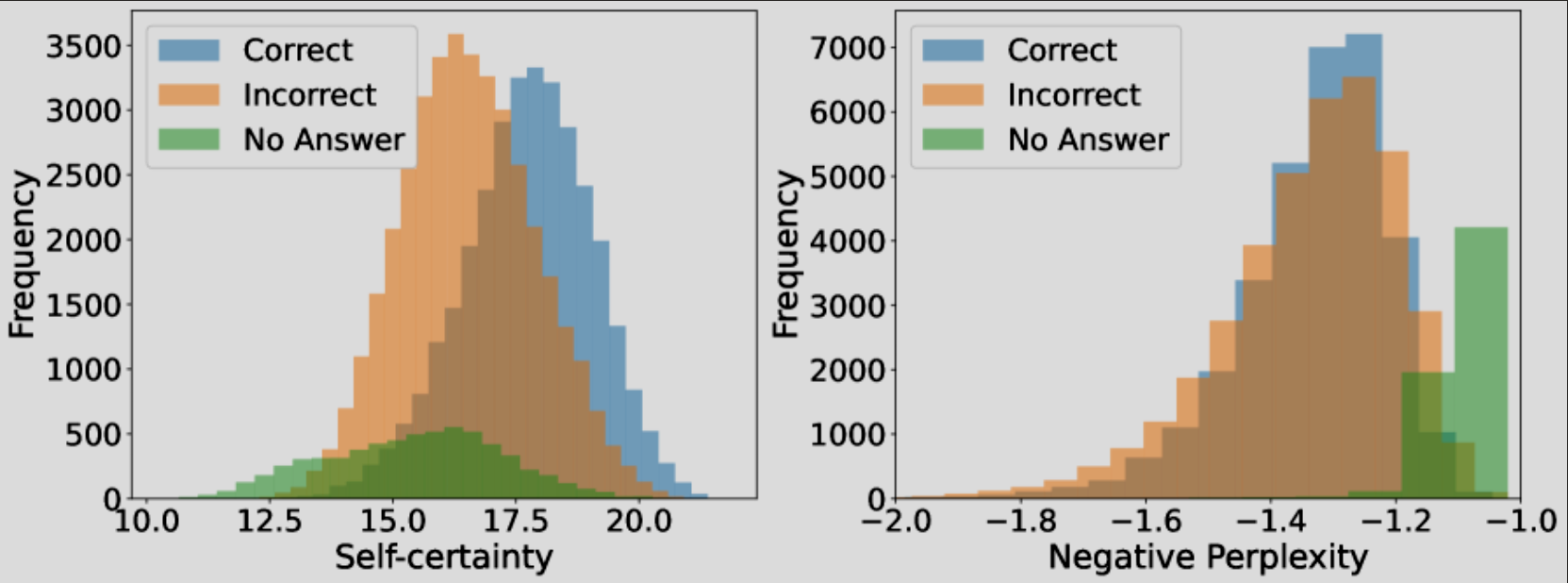
Self-Certainty (KL-Based Metric)
Average log probability only considers the chosen tokens. But what about the shape of the entire probability distribution at each step?
Self-certainty measures how "peaked" the model's token distributions are using KL divergence:
\[\text{Self-Certainty} = - \frac{1}{n_V} \sum_{i=1}^{n_X} \sum_{j=1}^{V_X} \log \Big( V \cdot p\big(j \mid x, y \le i\big) \Big)\]where
\[p(j \mid x, y_{\le i}) \;=\; \text{full token distribution at step } i\] \[V=\text{Vocabulary Size}\] \[p(j)=\tfrac{1}{V} \;\Rightarrow\; \log(V p(j)) = 0 \quad (\text{uniform} \;\Rightarrow\; \text{uncertain})\] \[\text{peaked } p \;\Rightarrow\; \log(V p(j)) > 0 \quad (\text{confident})\] \[\text{We divide by } \frac{1}{n_v} \text{to make the metric independent of sequence length} \\ \text{where } n_v \text{is the number of tokens produced}\]Intuitively:
- Flat distribution → uncertain model → lower self-certainty
- Peaked distribution → confident model → higher self-certainty
Why this works: KL divergence measures how far the probability distribution deviates from uniform. A confident model places most probability mass on a few tokens (high KL), while an uncertain model spreads probability across many tokens (low KL).
The most uncertain model gives the uniform distribution
Research shows that self-certainty more effectively distinguishes correct from incorrect samples, especially at higher N values, compared to simple AvgLogP.
Enhanced Methods: Combining Self-Certainty with Voting
For closed-ended questions like math problems, we can combine self-certainty scoring with voting mechanisms:
Borda Count Voting:
- Generate N responses
- Rank all responses by their self-certainty scores
- Assign weighted votes based on rank (highest-ranked gets most votes)
- Select the answer with the most total votes
This approach leverages both the model's confidence (via self-certainty) and consensus (via voting), providing a robust selection mechanism without requiring external reward models.
Empirical Results
Research demonstrates that KL-divergence-inspired distributional confidence metrics:
- More effectively distinguish correct samples from incorrect ones
- Achieve superior accuracy at higher N values
- Outperform simple token-probability metrics
Conclusion
Reward-free comparison methods offer a compelling alternative to traditional critic-model approaches:
Advantages:
- No need to train expensive critic models
- No inference-time overhead from running separate models
- Immune to reward hacking
- Leverage the base model's own uncertainty estimates
Based on: https://arxiv.org/pdf/2502.18581
My Naive implementation: Google Colab